Self-Supervised Learning (SSL) Deep Dive

14 Sep, 2025

Unlocking the Power of Self-Supervised Learning (SSL)

Understanding the Math, Principles, and Applications

Self-Supervised Learning (SSL) has rapidly become one of the most significant breakthroughs in the AI field, enabling data-efficient, scalable, and flexible models. SSL leverages the vast amounts of unlabeled data that exist across domains like computer vision, natural language processing (NLP), and speech recognition. This blog explores the mathematical intuition, the first principles behind SSL, and how it's shaping the future of AI.

Let’s dive into the fundamental principles of SSL, dissect the key components like contrastive learning, predictive coding, and Contrastive Predictive Coding (CPC), and look at their practical applications in real-world AI systems.

The Core of Self-Supervised Learning

What is Self-Supervised Learning?

Self-Supervised Learning is a paradigm where the model learns useful representations from unlabeled data by creating pretext tasks. Unlike supervised learning, where labels are manually provided, SSL enables the model to generate its own supervisory signals based on inherent structures in the data. The model is tasked with predicting a part of the input data, like filling in missing values or predicting future sequences.

Example:

In computer vision, SSL methods like SimCLR train a model to recognize similar images without explicit labels.
In NLP, models like BERT predict missing words or phrases in sentences.

SSL is data-efficient, making it incredibly useful when large labeled datasets are hard to obtain. But how does SSL learn from unlabeled data? Let's dig into the math behind it.

Mathematical Foundation: Contrastive Learning

The Power of Contrastive Learning

One of the pillars of SSL is contrastive learning. The fundamental idea behind contrastive learning is to map similar data points to nearby locations in a latent space and push dissimilar ones further apart.

Positive and Negative Pairs

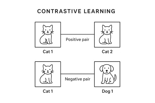
The core idea behind contrastive learning is the distinction between positive pairs (similar data points) and negative pairs (dissimilar data points). Consider the following:

Positive pair: Two augmented versions of the same image (e.g., a cropped and rotated version of the same photo).
Negative pair: Two images from different classes (e.g., a cat and a dog).

Diagram: Contrastive Learning in Latent Space

Contrastive Learning

Predictive Coding: Learning Through Prediction

What is Predictive Coding?

Predictive coding involves predicting future data or missing parts of the current data from what is already known. This technique helps the model learn temporal or spatial relationships in data.

For example:

In video prediction, a model learns to predict the next frame in a video sequence given the previous frames.
In text, it can predict the next word or sentence given the current context.

Mathematical Formulation

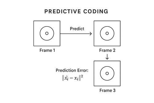
The goal of predictive coding is to minimize the difference between the predicted feature ( ${\hat{x}}_{i}$ ) and the actual feature ( $x_{i}$ ). This can be done using a simple mean squared error loss function:

L_{predictive} = \sum_{i} ‖ {\hat{x}}_{i} - x_{i} ‖^{2}

Where:

${\hat{x}}_{i}$ is the predicted feature.
$x_{i}$ is the actual feature.

Diagram: Predictive Coding in Action

In the context of video, we are predicting the next frame:

Predictive Coding

Contrastive Predictive Coding (CPC): The Best of Both Worlds

What is CPC?

Contrastive Predictive Coding (CPC) combines contrastive learning and predictive coding. It involves predicting the future context of the data while using a contrastive loss to distinguish between correct and incorrect predictions.

Mathematical Formulation of CPC

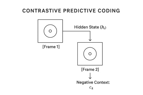
Let $h_{t}$ be the hidden representation at time $t$ , and $c_{t}$ the context or future representation at time $t + 1$ . The CPC loss is formulated as:

L_{CPC} = - \log \frac{\exp (sim (h_{t}, c_{t}) / τ)}{\sum_{k = 1}^{N} \exp (sim (h_{t}, c_{k}) / τ)}

Where:

$h_{t}$ is the hidden state at time $t$ .
$c_{t}$ is the context (future state) at time $t + 1$ .
The loss function encourages the model to predict the future by maximizing the similarity between $h_{t}$ and $c_{t}$ .

Diagram: Contrastive Predictive Coding in Video

Contrastive Predictive Coding

Code Implementation

Imports and Setup

import torch
import torch.nn as nn
import torch.nn.functional as F
import torch.optim as optim
from torchvision import datasets, transforms, models
from torch.utils.data import DataLoader

Data Augmentation for SSL

transform = transforms.Compose([
    transforms.RandomResizedCrop(224),
    transforms.RandomHorizontalFlip(),
    transforms.ColorJitter(0.4, 0.4, 0.4, 0.1),
    transforms.ToTensor(),
    transforms.Normalize(mean=[0.485, 0.456, 0.406],
                         std=[0.229, 0.224, 0.225])
])

train_dataset = datasets.CIFAR10(root='./data', train=True, download=True, transform=transform)
train_loader = DataLoader(train_dataset, batch_size=64, shuffle=True, drop_last=True)

Model Architecture

NOTE: We'll use a ResNet-18 backbone and add a projection head to map features into a lower-dimensional latent space for contrastive loss.

class ContrastiveModel(nn.Module):
    def __init__(self, base_model):
        super().__init__()
        self.encoder = base_model
        self.projector = nn.Sequential(
            nn.Linear(512, 256),
            nn.ReLU(),
            nn.Linear(256, 128)
        )

    def forward(self, x):
        features = self.encoder(x)
        projections = self.projector(features)
        return F.normalize(projections, dim=1)

Contrastive Loss (InfoNCE)

We use the InfoNCE loss, which encourages the model to align positive pairs and repel negative ones in the latent space.

Mathematical Formulation

The loss for a pair of embeddings $z_{i}$ and $z_{j}$ is defined as:

ℒ_{i, j} = - \log \frac{\exp (sim (z_{i}, z_{j}) / τ)}{\sum_{k = 1}^{2 N} 1_{[k \neq i]} \exp (sim (z_{i}, z_{k}) / τ)}

Where:

$sim (a, b) = \frac{a^{⊤} b}{‖ a ‖ ‖ b ‖}$ is the cosine similarity between two vectors.
$τ$ is the temperature hyperparameter that controls the sharpness of the distribution.
$2 N$ is the total number of samples (i.e., positive + negative pairs) in the batch.
$1_{[k \neq i]}$ is an indicator function that excludes the positive pair from the denominator.

The goal is to maximize the similarity between $z_{i}$ and its positive counterpart $z_{j}$ , while minimizing similarity with all other samples $z_{k}$ for $k \neq i$ .

def contrastive_loss(features, temperature=0.5):
    batch_size = features.shape[0] // 2
    labels = torch.cat([torch.arange(batch_size)] * 2, dim=0)
    labels = (labels.unsqueeze(0) == labels.unsqueeze(1)).float().cuda()

    similarity_matrix = F.cosine_similarity(features.unsqueeze(1), features.unsqueeze(0), dim=2)

    # Mask out self-contrast cases
    mask = torch.eye(labels.shape[0], dtype=torch.bool).cuda()
    labels = labels[~mask].view(labels.shape[0], -1)
    similarity_matrix = similarity_matrix[~mask].view(similarity_matrix.shape[0], -1)

    positives = similarity_matrix[labels.bool()].view(labels.shape[0], -1)
    negatives = similarity_matrix[~labels.bool()].view(similarity_matrix.shape[0], -1)

    logits = torch.cat([positives, negatives], dim=1)
    labels = torch.zeros(logits.shape[0], dtype=torch.long).cuda()

    logits /= temperature
    return F.cross_entropy(logits, labels)

Training Loop

optimizer = optim.Adam(model.parameters(), lr=3e-4)
epochs = 20

for epoch in range(epochs):
    model.train()
    total_loss = 0

    for (images, _) in train_loader:
        images = images.cuda()

        # Generate two augmented views for each image
        x1, x2 = images, images.clone()

        # Concatenate for a single forward pass
        inputs = torch.cat([x1, x2], dim=0)
        features = model(inputs)

        # Compute contrastive loss
        loss = contrastive_loss(features)

        optimizer.zero_grad()
        loss.backward()
        optimizer.step()

        total_loss += loss.item()

    avg_loss = total_loss / len(train_loader)
    print(f"Epoch [{epoch+1}/{epochs}], Loss: {avg_loss:.4f}")

Applications of SSL

SSL techniques are revolutionizing practical applications across AI fields:

Computer Vision: SSL methods like SimCLR are widely used for tasks such as image recognition and object detection, where the model learns to group similar images together, even without labeled data.
Natural Language Processing (NLP): Models like BERT and GPT use SSL by predicting masked tokens in a sentence, leading to the development of powerful language models that understand the structure of human language.
Speech Recognition: SSL helps in learning speech representations from raw audio, improving tasks like automatic speech recognition (ASR) and speaker identification.

Conclusion: The Future of Self-Supervised Learning

Self-Supervised Learning is a transformative force in AI. By enabling models to learn from unlabeled data, SSL reduces the reliance on expensive manual labeling and helps us leverage the vast amounts of data that are freely available. The combination of contrastive learning and predictive coding forms a powerful framework that enables models to understand the structure of the world without supervision.

With its growing applications in vision, language, and speech, SSL is set to revolutionize how we train AI systems and unlock generalized models capable of learning from any data.